Real-time voyage optimisation for CII compliance: notes from the SOOS programme

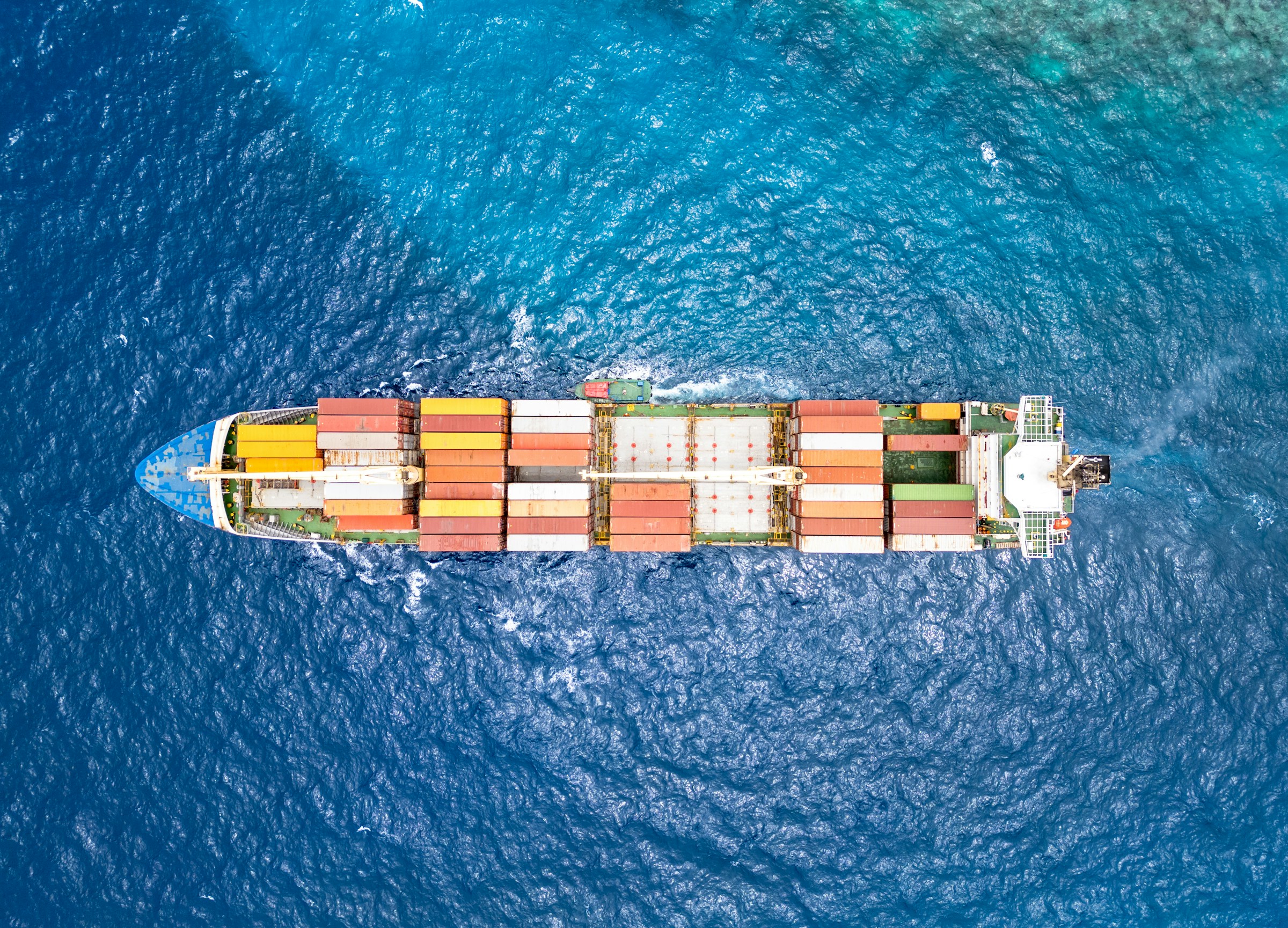
• ·The IMO's 2023 GHG Strategy (MEPC.377(80)) targets a roughly 30% absolute drop in shipping emissions by 2030. For an existing fleet, hardware retrofits get you 5 to 15% (DnV 2022); the rest must come from how the ship is operated.
• ·SOOS is not a routing app. It is a coupled hydrodynamics + optimisation stack: CFD calm-water resistance, semi-empirical wind loads, Salvesen-1978 added resistance in waves, trim-via-centre-of-gravity, and a Vectorized Simulated Annealing layer over the route geometry.
• ·"Real-time" means seconds, not minutes — the model has to re-plan as forecasts update and as fuel burn shifts the centre of gravity. We precompute the expensive physics offline and re-use it inside the optimiser.
• ·On a 712 TEU geared containership in synthetic Atlantic conditions, SOOS converged inside 100 epochs and saved 8 to 9% of voyage fuel versus the great-circle direct route. With an obstacle inserted in the route grid, the saving held at roughly 8%.
• ·Fuel saved is emissions saved. For a CII-regulated containership, the same 8 to 9% is the difference between staying inside the operating band and entering corrective-action territory.

Why the IMO 2030 target is an operational problem, not a hardware problem

The IMO's 2023 GHG Strategy (Resolution MEPC.377(80)) commits the maritime sector to a roughly 30% absolute reduction in well-to-wake emissions by 2030 relative to 2008 levels. The international fleet today emits about 681 megatonnes of CO2 a year. Hardware retrofits — coatings, hull-form tweaks, propeller polishing — buy you 5 to 15% per vessel. Operational measures must close the rest of the gap.

The arithmetic is unforgiving for an existing containership. DnV's 2022 maritime forecast put the per-vessel hydrodynamic envelope at 5 to 15% and the operational envelope (speed management, fleet planning, weather routing — what DnV calls logistics and digitalisation) at more than 20%. A new build can be designed for the new band; a 2010s containership cannot. Its operator has to find the missing percentage points in how the vessel is sailed, not how it is built. That is the boundary condition we wrote SOOS against. Add the macro context — bunker prices held high by the war in Ukraine and Middle East shipping disruptions, and the World Shipping Council reporting more than 3,113 containers lost overboard in 2020 to 2021 — and the operational case stops being academic. Safer voyages also burn less fuel.

What "real-time" actually demands of the model

A real-time voyage optimiser has to compute four things faster than a forecast updates: the calm-water power needed at any speed and trim, the wind loads on the above-waterline projection, the added resistance the seaway is imposing on the hull, and the response of the centre of gravity as fuel and ballast move around the vessel.

The honest version is that none of these can be done in real time from first principles on a ship's bridge computer. CFD on a containership in waves is hours per case at best. So the architecture is the inverse: precompute the expensive physics offline at high fidelity, distil it into a small set of coefficients and lookup surfaces, and have the optimiser query those surfaces inside its inner loop. The on-board cost then collapses to interpolation plus the optimisation itself. Where SOOS earns its keep is in being honest about which simplifications hold under operational forecasts and which do not — which is why the methods paper at IMDC 2024 is half about the simplifications, and the systems paper at ICCAS / RINA later the same year is about the cases where the simplifications break down.

The four hydrodynamic ingredients

Each layer of the stack has its own validation history and its own cost-accuracy compromise. We chose them on the basis of what gives the best signal per second of compute on a 120-metre containership.

Calm-water resistance from CFD, not regression

For the 712 TEU case, we ran the calm-water resistance in Simerics MP — a RANS solver with a marine template — swept across speeds at the design trim of 0.2° by stern. The output was fitted as a third-order polynomial in speed, forced through the origin, and converted to power via a propulsive coefficient of 0.656 derived from the same campaign.

The practical reason for going to CFD instead of a Holtrop-Mennen-style regression is that those regressions are calibrated on hull families that no longer represent the modern containership population. The accuracy gain matters because every downstream layer — wind, waves, trim — is a perturbation on the calm-water number, and a wrong baseline propagates everywhere. The cost is one CFD campaign per vessel, per loading condition that operations actually uses, run once. That is a one-off bill the fleet owner pays in exchange for a defensible power curve.

Wind loads, semi-empirical first

Wind loads come from the Isherwood (1972), Gould (1982), and Blendermann (1994) family of semi-empirical formulations, applied to the projected lateral and transverse areas above the waterline. On most ship types the wind contribution is around 2% of total resistance. On a containership stacked six-high above deck — roughly 60% of the boxes are above the main deck — it can reach 10%.

We default to the semi-empirical route for two reasons. First, the dependence on heading is well-characterised across the Isherwood-Gould-Blendermann tradition, so the lookup is small and stable. Second, the wind-resistance signal is dominated by the projected area, and the projected area is known exactly from the loading condition. CFD can do better — we have run it and we say so in the paper — but the marginal gain rarely justifies the marginal cost on a vessel whose dominant uncertainty is the forecast wind itself, not the load coefficient. When the dominant uncertainty is somewhere else, you spend the CFD budget there.

Added resistance in waves: Salvesen-1978 over Gerritsma-Beukelman

Added resistance in irregular waves is computed with the Salvesen (1978) formulation built on Frank's close-fit strip theory, with a short-wave correction. We compared it against Gerritsma-Beukelman (1979); both agree in head waves, but Gerritsma-Beukelman drifts in quartering seas in a way our seagoing experience says is wrong, so we use Salvesen.

To put a number on it: for the 712 TEU case at top speed (Froude number 0.26), facing the most statistically frequent Atlantic train (significant wave height of 1.25 metres, peak period of 9 seconds, head seas), Salvesen returns an added resistance of 13.42 kilonewtons. That is 1.7% of total resistance, or 2.9% of the residuary resistance. Small in flat conditions; in storm conditions it dominates. The strip-theory transfer functions are precomputed across heading and frequency and looked up inside the optimiser. Speed loss in waves falls out of the same lookup, so we do not over-predict the speed the engine can hold.

Trim and the moving centre of gravity

Trim is the cheapest available lever. Small changes in longitudinal centre of gravity move the dynamic trim by tenths of a degree and reclaim measurable kilowatts at the propeller. SOOS tracks the instantaneous centre of gravity from the discrete weights aboard — fuel, ballast, cargo, crew — and computes the trim correction needed via the unit moment to change trim.

The point of computing this in real time is that the operator does not actually know the centre of gravity at any given moment. The departure-condition stability book is a snapshot. Hours later, fuel has been burned out of the aft tanks, ballast has been adjusted, and the trim is no longer optimal. SOOS recomputes the optimal trim against the current loading and prompts a ballast transfer when the gain justifies the operational cost. On the 712 TEU case the ideal trim was 0.2° by stern — the same value used in the calm-water CFD campaign — but the more interesting fact is that this number changes across the voyage.

Why simulated annealing is the right routing layer

The route-geometry search space — find the sequence of waypoints that minimises fuel between two ports under a forecast meteocean field, while respecting land and traffic exclusions — is non-convex, has hard boundaries, and is not differentiable across those boundaries. Simulated annealing tolerates all three. We use a vectorised variant adapted from Maurício and Moreira (2022), originally developed for sailboat routing under non-uniform wind fields.

The mechanics are unromantic. SOOS represents a route as a chain of N − 1 waypoints between origin and destination. It generates a population of 200 candidate routes with random waypoint positions, evaluates the fuel for each by integrating the consumption rate along the leg, retains the best half, perturbs them with a spatial noise whose amplitude decays exponentially across epochs, and repeats. The decay schedule is the temperature analogue from classical annealing. Vectorisation means that the perturb-and-evaluate step runs in parallel across the whole population on commodity hardware. We capped at 750 epochs in the published case, but the optimiser converged inside 100 — which is the property you want, because the operator on the bridge will not wait for 750. The five-step heuristic is laid out fully in the IMDC 2024 paper; the relevant part for an operator is that there are no hyperparameters they need to tune.

The 712 TEU case — and what 8 to 9% really means

On a synthetic Atlantic field — uniform 23-knot wind from the west, a 2.14-knot west-going current, a 1.25 m / 10 s regular west swell, two ports about 215 km apart — SOOS routed the 712 TEU geared containership for 3.99 kg of fuel against 4.31 kg on the great-circle direct route. The saving was 8 to 9%.

The harder version of the same case had us insert an "island" exactly where the optimal route wanted to go. The optimiser detoured around it and still landed at 3.97 kg — an 8% saving. That is the property we cared about: the saving is not a fragile artefact of a friendly cost surface. It is robust to the kind of geographic constraint a real voyage actually has — a marine corridor, a fishing exclusion zone, a weather-routing waypoint imposed by a charterer. Multiply 8% across a fleet's annual bunker bill and the number stops being a curiosity. For a mid-size containership on a Mediterranean-Atlantic loop, an 8% voyage saving compounds to seven figures of avoided fuel cost per year, and it shifts the same vessel's CII rating by enough to matter at the next port-state inspection.

What we are not yet claiming

These results are preliminary. The environment is synthetic, not a hindcast. The optimiser has not been validated against sea-trial data on the case-study vessel. The anti-rolling-tank coupling described in the introduction of the IMDC 2024 paper is not yet wired into the optimiser. And the model assumes vessel heading equals course over ground, which is conservative in current but wrong in heavy weather.

The companion ICCAS / RINA paper from later in 2024 takes the next step: it sets the same SOOS stack against a real-case meteocean field from the MOHID large-circulation hydrodynamic model, and against a containership refit that converts an existing anti-heeling tank into an anti-rolling U-tank. That paper is where the systems-level story lives — coupling the routing layer to the on-board roll-stabilisation hardware, and asking whether a vessel that is more comfortable at any given speed is also a vessel that operates at speeds closer to its hydrodynamic optimum. The next milestone is the at-sea validation campaign. Until that is done, we will keep saying "the simulation says 8 to 9%" rather than "we save 8 to 9%". The two are not the same sentence.

Why this matters beyond one containership

Voyage optimisation is a generic decarbonisation lever. Any vessel that is large, fast, and operating against a forecastable meteocean field — containerships, RoRos, ferries, OSVs on long-distance steam-outs — has the same arithmetic available to it. The four physical ingredients are the same; only the coefficients and the optimiser cost surface change.

Hardware retrofits buy 5 to 15%. Operational measures, done well, can buy more than 20%. For an existing fleet under the 2030 IMO target, "done well" is not optional — and it is mostly software.

The harder problem, and the one we intend to keep working on, is the integration. A weather-routing tool that lives in a separate window from the engine-room console, or that asks the bridge officer to type forecasts into a spreadsheet, will not survive the second week of a voyage. SOOS is being built so that the calm-water curves, the wave responses, the wind loads, and the routing layer are one stack with one interface, and so that the operator can trust a single number on the screen. Whether we have got that right is what the sea trials are for.

Frequently asked questions

What is the Carbon Intensity Indicator (CII)?

The CII is an IMO operational metric, in force since January 2023, that rates a ship's annual carbon emissions per unit of transport work — grams of CO2 per tonne-mile. Each ship is given a letter rating A to E. Three consecutive C ratings, or a single E, require a corrective-action plan to be submitted to the flag state.

How is SOOS different from a commercial weather-routing service?

Commercial services typically optimise over a black-box ship model fitted to operational data. SOOS optimises over an open hydrodynamic model fitted from CFD and strip theory on the actual vessel. The difference matters when the loading condition or trim moves outside the operational envelope the black-box was fitted on — exactly when the largest fuel-saving opportunities tend to appear.

How much fuel can voyage optimisation realistically save?

On the synthetic Atlantic case in our IMDC 2024 paper, the saving was 8 to 9% versus the great-circle direct route. DnV's 2022 outlook puts the upper bound on operational measures at more than 20% across speed management, fleet planning, and weather routing combined. Single-voyage gains will sit somewhere inside that band, depending on route, season, and vessel type.

Is this approach only for containerships?

No. We tested SOOS on a 712 TEU geared containership because containerships are the highest emissions producers per nautical mile in the world fleet, but the four physical ingredients — calm-water resistance, wind loads, added resistance in waves, trim response — are generic. Tankers, bulkers, RoRos, and ferries each have their own coefficient sets but the same model architecture.

When will sea-trial validation be available?

The validation campaign is planned for the next phase of the SOOS programme, in coordination with the case-study vessel's operator. The companion ICCAS / RINA 2024 paper sets the framework for it. Until trials are complete, we describe SOOS as a methods study and not as an operational claim.